Course Instructors:
Prof. Dr. Saeed Asiri
- Office: 24E38
- Website: https://www.asiri.net
- WhatsApp: +966565555275
- Email: saeed@asiri.net
- Twitter: @drsaeedasiri
- Facebook: saeedasiri
Course Description:
Introduction, Laplace transforms , system transfer function (TF), constructing Block diagrams, state space equations of control systems. mathematical modeling of dynamic systems: mechanical, electrical, transient response of a system, Bode plots for system identification and stability, Nyquist diagram , stability of the system, Routh’s stability criterion, basic control actions, design the control systems in state space, using MATLAB to study any linear system.
Text Book: Modern Control Engineering, Katsuhiko Ogata, Fifth Edition
Reference: Control Systems Engineering, Nise.
How to Succeed
Accept that it is your responsibility to learn the material (in spite of the book or teacher)
Show up and become engaged with the topics
Your main homework assignment is to watch the video to understand the topic in advance so that you can collaborate in the class activities
Use you resources for help (internet, classmates, upperclassmen, faculty, the library)
Course Learning Objectives:
Conceptual:
- To learn how to model the system to be controlled in terms of a transfer function
- Understand the system’s behavior from the transfer function
- Learn how to use the feedback and a controller to alter the behavior of the system as d
ABET CLOs:
- Evaluate Laplace and Inverse Laplace Transformations.
- Understand how to get the transfer function (TF) of a physical system
- Identify specifications of a transient response of a second order system. (maximum overshoot, rise time, peak time, settling time)
- Determine the stability of the system using Routh’s stability criterion.
- Analyze a system error related to a transient response of a control system.
- Design a control system using basic control actions. (P., PI., PD., and PID control)
- Design a control system using root-locus method.
- Sketch Bode plots and use it for system identification and stability.
- Use Nyquist diagram to determine the stability of a closed loop system.
- Model and analyze the control systems in state space.
- Use MATLAB to study a linear system
Grading Policy:
Laboratory | 10% |
Quizzes | 40% |
Term Project | 10% |
Collaborative Learning Activities | 10% |
Final Opportunity To Shine | 30% |
Note: 75% attendance is required. No makeup for any quiz. Student must attend the laboratory to pass the course.
|
Month |
Su |
Mo |
Tu |
We |
Th |
Fr |
Sa |
TOPIC |
|
Jan |
14 |
15 |
16 |
17 |
18 |
19 |
20 |
Create Groups |
|
21 |
22 |
23 |
24 |
25 |
26 |
27 |
Introduction to Control System |
|
|
28 |
29 |
30 |
31 |
|
|
|
Transfer Functions, Block Diagrams, |
|
|
Feb |
|
|
|
|
1 |
2 |
3 |
Signal Flow and Mason’s Rule |
|
4 |
5 |
6 |
7 |
8 |
9 |
10 |
Mathematical Modeling of Mechanical |
|
|
11 |
12 |
13 |
14 |
15 |
16 |
17 |
Transient and Steady State Response |
|
|
18 |
19 |
20 |
21 |
22 |
23 |
24 |
Routh’s Stability Criterion |
|
|
25 |
26 |
27 |
28 |
29 |
|
|
Root Locus Analysis: General Rules |
|
|
march |
|
1 |
2 |
Bode Plots, Stability using Bode Plot |
||||
|
3 |
4 |
5 |
6 |
7 |
8 |
9 |
Advanced Bode Plot |
|
|
10 |
11 |
12 |
13 |
14 |
15 |
16 |
Nyquist Plot Analysis and Stability |
|
|
17 |
18 |
19 |
20 |
21 |
22 |
23 |
System Modeling in State Space |
|
|
24 |
25 |
26 |
27 |
28 |
29 |
30 |
Observability and Controllability |
لا. | عنوان | بي دي إف | فيديو |
| 0 | تشجيع لأسلوب التعلم التعاوني | ن | ن |
| 1 | مساعدة في التحكم | انقر هنا | انقر هنا |
| 2 | وظائف النقل، والتغيرات الكتلية، | انقر هنا | انقر هنا |
| 3 | تدفق وقاعدة ماسون | انقر هنا | انقر هنا |
| 4 | النمذجة الرياضية للأنظمة الميكانيكية والكهربائية والخطية | انقر هنا | انقر هنا |
| 5 | مقبول الاستقرار روث | انقر هنا | انقر هنا |
| 6 | قم بتسجيل الدخول إلى اللعبة والثابتة لأنظمة المشاركة الأولى والأعلى | انقر هنا | انقر هنا |
| 7 | النظام وأخطاء الحالة الثابتة مركز التحكم | انقر هنا | انقر هنا |
| 8 | تحديد موضع RGB: متطلبات عامة لإنشاء موقع RGB ومخططات موضع RGB باستخدام MATLAB | انقر هنا | انقر هنا |
| 9 | موسيات وهمية، لاستخدامها في تحقيق أهدافها | انقر هنا | انقر هنا |
| 10 | التقنيات المستخدمة للتردد باستخدام مخططات Bode وNyquist | انقر هنا | انقر هنا |
| 11 | اعتماد النظام في مساحة الدولة | انقر هنا | انقر هنا |
General Format for Lab Reports
• TITLE PAGE (l)
Report title, course, your name, date lab performed, date lab due, date report submitted.
• OBJECTIVE OF THE EXPERIMENT (1)
Statement of objective or purpose of the experiment/lab
• THEORY/EQUATIONS USED (3) List the equations used for your lab calculations (if any).
• SAMPLE CALCULATIONS/DATA GENERATED (5) A sample of the calculations you performed to get your results.
• PROGRAM LISTING (5) A listing of your MATLAB program (if any)
• CONCLUSIONS/ANSWERS TO QUESTIONS (5)
List your conclusions. Include answers to all questions asked in the lab handout here. Make sure your answers are well explained
• RESULTS(S)
Your results, any problems you have had in this lab, your comments on the lab
• CLASS PARTICIPATION (5) (experimental labs)
Your active participation in the lab is crucial to the experience. Additional unique insight presented in your report may also be represented here.
Please remember, it’s what you put in your report that counts and not how much you put in it. Some of these labs require you to turn in MATLAB plots, do not turn in all that you have printed out, but only what has been asked for. If you are not sure about what you need to turn in, please ask the engineer. Once again, remember that most of the points that you get for a lab come from your answers to the questions in the lab handout.
Points may be taken off for grammar/spelling and sloppy presentation. The reports should be typewritten. PCs are available in the computer lab for word processing
• All students should know how to operate the equipment in the lab and take part in the execution of the lab. It will be reflected in your grades.
• Question/s about the labs will be asked on exams. Not specifics, but concepts, methods and techniques.
Virtual Experiments using SIMULINK.
| Week No. | LAB. Topic | Handout |
| 1 | Introduction to SIMULINK | Click here |
| 2 | Block Diagram Reduction I | Click here |
| 3 | TRANSFER FUNCTION SIMPLIFICATION AND SOLUTION | Click here |
| 4 | Transfer Function of LTI Systems | Click here |
| 5 | MATHEMATICAL MODELING OF MECHANICAL SYSTEMS | Click here |
| 6 | Routh’s Stability Criterion | Click here |
| 7 | System Frequency of First Order System | Click here |
| 8 | System Frequency of Second Order System | Click here |
| 9 | PID CONTROL | Click here |
| 10 | FREQUENCY RESPONSE ANALYSIS USING BODE PLOT | Click here |
| 11 | FREQUENCY RESPONSE ANALYSIS USING POLAR PLOT | Click here |
| 12 | Modeling in State Space | Click here |
Lab Overview:
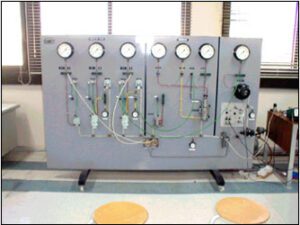
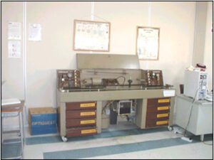
This laboratory covers the experimental aspects of the topic of automatic control within the field of mechanical engineering applications. The main interest is in modeling and simulation of dynamic systems with the aim of emphasizing the main concepts and training the students to conduct experiments and correlate the results. The same problem can be solved on more than one apparatus. This results in better appreciation of the problems of experimental work and helps furnish a deeper understanding of the subjects dealt with. The equipment existing in the laboratory serves both introductory and higher level courses suitable for undergraduates and postgraduates respectively. These include a pneumatic simulator comprising 3 first-order processors, together with three controllers, two analog computers containing six summers and six integrators, together with nonlinear and logic elements. In fluid dynamics there are three units; water level control, fluid power pack and hydraulic servo speed control. Also, measuring and indicating units are available which include paper recorder, x-y recorders and four-channel oscilloscopes.
Pic 1
Pic 2

MENG 366: Automatic Control
Project weight: 10% of the final grade
This is an open-ended project, where each group designs its own project according to some restrictions and requirements. The project includes:
- Written report.
- Poster.
- Oral Presentation.
- Physical model to validate the mathematical model.
Each group should work independently but can share their experience by teaching their colleagues some of their useful skills. Groups should NOT have similar designs, even if the parameters are different.
Students, in groups of no more than five, are to model, analyze, and control a physical system using the tools and techniques learned in this class. It is expected that students will analyze their system using both analytical techniques as well as numerical methods.
The goal of this project is to illustrate the modeling, analysis, control and simulation techniques learned in this class on a physical system. A significant component of the project is to model and analyze models of any physical system and then to build the suitable control action. In this way, students can be exposed to the influence of control action on the system behavior.
Each project must allow for the following:
- The model must admit a closed-form solution (i.e., it must be linear, with constant coefficients).
2.The control action must be considered.
3.You must present both analytical and numerical results
Each report will be organized as follows:
- Introduction: what are you doing and what information will you obtain;
Modeling: identify appropriate modeling assumptions and develop the equations of motion which correspond to the different sets of assumptions;
2. Linear Analysis: linearize the above models about some operating point and analyze the resulting behavior predicted by each model;
Simulation: use MATLAB and/or SIMULINK to verify the analytical predictions of both the qualitative and quantitative behavior of the system with and with out control system.
3. Conclusions: model extensions, including the validity of the constitutive assumptions, discussion of results, effect of modeling assumptions, effect of choosing a specific control action and varying the control gain etc.
4. (10 points) On Sunday, MARCH. 10: Final design drawings are due. Show Eng. Hafiz a clear drawing of your design before this date, and get the approval by this date.
The idea is for you to figure out how your system is going to behave. For example, what happens as the parameters vary, what happens when the control gain is varied, how will the predicted dynamics vary with modeling assumptions, etc. You will employ both analytical techniques (modeling and solving the equations in closed-form) as well as numerical methods (MATLAB and/or SIMULINK) to get the system response.
